DETR on SPECT images: automatic RSI computation to assess residual thyroid tissue after thyroidectomy
An explainer of an IEEE SSP 2023 paper: DETR detects the thyroid and shoulders on I-131 SPECT images and automatically computes the RSI index to diagnose residual thyroid tissue (F1 0.91). Detailed analysis of every experiment, formula and figure.
TL;DR: The paper “Utilizing DETR model on SPECT image to assess remaining thyroid tissues post-thyroidectomy” (IEEE SSP 2023, pp. 537–541) is the follow-up to the NICS 2022 study. Instead of having a CNN answer “residual tissue or not” directly, the authors use a DETR (Detection Transformer) model to localize the thyroid and the shoulder regions on I-131 SPECT images, then compute a quantitative number that physicians can understand: the RSI (Radioiodine Scan Index), the ratio of radioactive uptake between the neck region and the shoulder region. A logistic regression model based on RSI achieves a diagnostic F1 = 0.91 (Accuracy 0.96, Precision 0.86, Recall 0.95), better than direct classification with ResNet-50 (F1 = 0.88). The paper also proposes a new evaluation metric (RSIA) for selecting the detection model according to the actual clinical goal rather than looking at mAP alone.
Paper at a glance
| Item | Details |
|---|---|
| Title | Utilizing DETR model on SPECT image to assess remaining thyroid tissues post-thyroidectomy |
| Authors | Minh Lai Phu, Thanh Trung Nguyen, Thanh Vinh Pham, Thai Ha Nguyen, Duc Thuc Pham, Minh Duc Chu, Chi Thanh Nguyen, Quoc Long Tran, Duc Thuan Nguyen, Ngoc Ha Le, Hong Son Mai, Thi Nhung Nguyen, Thi Phuong Nguyen, Quoc Khanh Le, Nam Thang Dang |
| Affiliations | Department of Electronics, School of Electrical and Electronic Engineering, Hanoi University of Science and Technology (HUST); Faculty of Information Technology, VNU University of Engineering and Technology (UET); Departments of Medical Equipment and Nuclear Medicine, 108 Military Central Hospital; Institute of Information Technology, Academy of Military Science and Technology |
| Conference | SSP 2023, pp. 537–541 |
| Funding | Project TXTCN.21.23, Vietnam National University, Hanoi |
| Task | (1) Object detection: residual thyroid and shoulder region; (2) Binary diagnosis of residual tissue / no residual tissue from the RSI index |
| Model | DETR (ResNet-50 backbone) + logistic regression on RSI |
| Main results | F1 0.91 · Thyroid [email protected] = 0.73 · Shoulder [email protected] = 0.604 · RSIA = 0.457 |
From “classification” to “detection + measurement”: why change direction?
In the NICS 2022 paper, a ResNet-50 model looked at the whole image and returned a label. This approach has two weaknesses when brought into the clinic:
- Hard to explain. The model says “residual tissue” but not where or how much. Heatmaps help to some extent, but they are still indirect guesses.
- It does not match the physician's workflow. Nuclear medicine physicians usually compare the radioactivity concentration in the thyroid bed with a background region to make an assessment. A ratio like that is easy to double-check, easy to threshold and easy to compare across scans.
The SSP 2023 paper follows exactly that workflow: find regions → measure uptake → compute a ratio → make a decision. The deep learning model only handles the “find regions” part, while the decision is a transparent formula plus a single-variable logistic model.
The pipeline at a glance
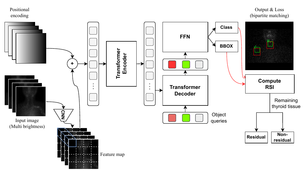
Figure 2 (from the paper). Red boxes are model predictions, green boxes are ground truth labels.
flowchart LR
    A[Whole-body scan<br/>256×1024] --> B[Crop head – neck region<br/>256×256]
    B --> C[Create 4 versions<br/>at different brightness]
    C --> D[DETR<br/>ResNet-50 + Transformer]
    D --> E[Thyroid box B_T]
    D --> F[Shoulder box B_S]
    E --> G["Compute RSI = U(E_T) / U(E_S)"]
    F --> G
    G --> H[Logistic regression]
    H --> I{Residual tissue?}
Data and preprocessing
The MCHSP400 dataset
Physicians at the Department of Nuclear Medicine, 108 Military Central Hospital collected and labeled the MCHSP400 dataset. The portion used for the experiments contains 396 cases of I-131 SPECT scintigraphy, each with:
- a diagnostic label of residual tissue (positive / residual) or no residual tissue (negative / non-residual);
- bounding boxes for the thyroid region (neck region) and the shoulder region.
An analysis of box sizes shows that most objects are small or medium, which is a hard case for many detection models. All data were collected with the permission of 108 Military Central Hospital.
| Split | Cases | Role |
|---|---|---|
| Train | 278 | Model training |
| Validation | 79 | Selecting the best model (by mAP or by RSIA) |
| Test | 39 | Final evaluation on unseen data |
| Total | 396 |
Step 1: Crop the head – neck region
Whole-body scans are 256×1024. Besides the thyroid, the image contains many other iodine-uptake regions such as the salivary glands, stomach and bladder. For this task they are just noise. The image is cropped to 256×256, keeping only the head – neck – shoulder region, so the model is not “distracted” by unrelated organs.
Step 2: Multi-brightness images
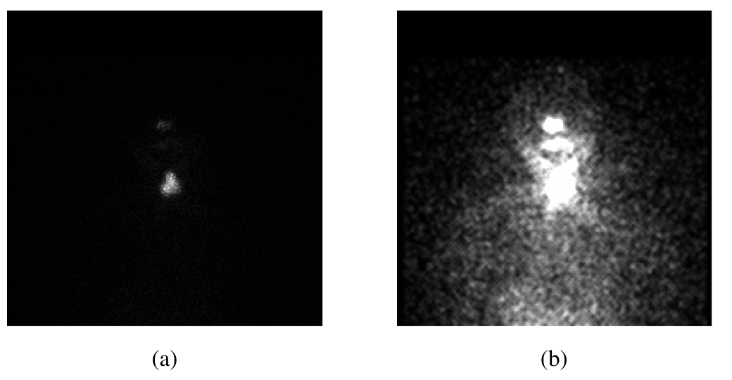
Figure 1 (from the paper). (a) Original image, body outline unclear. (b) Brightened image, body outline clearly visible.
SPECT images have a highly skewed dynamic range: regions of strong uptake (residual thyroid) are glaringly bright, while the rest of the body has only a few scattered photons and looks almost black. Using only the original image, the model can barely see the shoulders, because the shoulders do not take up iodine; they only show up as a faint background region.
The paper's solution is to create multiple brightness versions of the same image and stack them as input channels. The idea is similar to how radiologists adjust the “window” (window/level) when reading CT: each window highlights a different kind of detail.
A simple way to implement this transform (for illustration) is to multiply the intensity by different gains and then clip:
The model input is then a -channel tensor . Channel (the original image) keeps information about the strong uptake spot (the thyroid), while the brighter channels reveal the body outline and shoulders. The paper tests and picks (see Experiment 3).
Why do ordinary CNNs struggle?
CNN-based detection models such as Faster R-CNN and YOLOv7 consist of a feature extraction network (the backbone, usually pretrained on ImageNet) and subsequent layers that predict boxes. CNN backbones are very good at capturing local features: edges, textures, bright blobs.
The problem is that CNNs use many pooling / stride layers to shrink the feature maps. This reduces computation but gradually loses the global spatial relationships between distant regions of the image.
In this task, global relationships are the main clue:
- In cases where the thyroid tissue was completely removed, the neck region has almost nothing bright. The model has to infer the location of the thyroid bed from the body shape and its position relative to the shoulders.
- The shoulders do not take up iodine and have almost no texture of their own. Their position can only be inferred from the body outline and their relationship to the neck and head.
In other words, the model needs to answer questions like “where are the shoulders relative to the neck?”. That is a long-range relationship, exactly what the Transformer's attention mechanism handles well.
How does DETR work?
DETR (DEtection TRansformer) was introduced by Carion et al. (Facebook AI) at ECCV 2020. It treats detection as set prediction: the model directly outputs a set of (class, box) pairs, with no anchor boxes and no NMS (non-maximum suppression) post-processing step.
1. CNN backbone and positional encoding
The input image passes through ResNet-50 to produce a feature map . This map is flattened into “tokens”. Because a Transformer does not inherently know token positions, DETR adds a sine – cosine positional encoding (following Vaswani et al., 2017):
DETR applies this formula separately to the axis and the axis and concatenates the results, so each token “knows” which row and column it is in.
2. Transformer encoder: self-attention
Each encoder layer lets every position look at every other position through self-attention:
where are linear projections of the tokens. The weights indicate how much one position “attends to” another. A token in the shoulder region can look directly at a token in the neck region, even though the two regions are half an image apart. This is why DETR captures the global spatial relationships that CNNs tend to lose.
3. Transformer decoder and object queries
The decoder takes learned vectors called object queries (the original DETR paper uses ). Each query is like an “empty slot” asking: “is there an object in the image that corresponds to me?”. Through cross-attention layers over the encoder output, each query becomes an embedding, and then an FFN (feed-forward network) predicts:
- the class : thyroid, shoulder, or (“no object”);
- the box , normalized to .
4. Bipartite matching and the Hungarian loss
Because the output is an unordered set of predictions, DETR needs to know which prediction corresponds to which label. Let be the set of ground truth labels (padded with to elements). DETR finds the permutation with the lowest matching cost using the Hungarian algorithm:
Once matched, the model is trained with the Hungarian loss:
where the box loss is a combination of L1 and Generalized IoU:
where is the smallest box enclosing both and (the original DETR uses , ).
What this means in practice: one-to-one matching forces each real object to be “claimed” by exactly one query. As a result, DETR does not produce many overlapping boxes and does not need NMS. This is what the paper describes as “a bipartite loss that explicitly assigns each predicted box to a ground truth box or an empty box”.
Why did the paper choose DETR?
According to the authors:
- DETR overcomes the weakness of CNNs in capturing spatial relationships.
- Its prediction speed is faster than two-stage models such as Faster R-CNN and Mask R-CNN.
- It works well with the small and medium objects in this dataset.
- It does not fix the input image size; 256×256 or 512×512 can both be used.
Additional note from the author of this post: On natural images (COCO), the original DETR is generally known to be weaker on small objects and slow to converge. In this task, “small” refers to relative size within a 256×256 image, and there are very few objects per image (one thyroid, two shoulders), so DETR's advantage in global relationships outweighs that weakness.
The RSI index: turning boxes into a diagnostic number
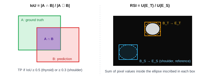
RSI (Radioiodine Scan Index) measures how many times more radioiodine the neck region takes up than a background region. The background region chosen is the shoulder, because the shoulder is close to the neck, has a similar soft-tissue depth, but contains no thyroid tissue.
The formula
For each box (the thyroid box or the shoulder box ), take the box's inscribed ellipse . If the box has center , width and height , then:
The uptake in a region is the sum of pixel values in that region:
Applied to the shoulder ellipse:
And RSI is the ratio of uptake in the thyroid to uptake in the shoulder:
Here is the pixel value at (photon counts on the original image), and are the ellipses inscribed in the thyroid box and the shoulder box.
Why ellipses, and why divide by the shoulder?
- Ellipse instead of rectangle: the thyroid and shoulder regions are round to oval in shape. The four corners of a box are mostly background, and adding them in would “dilute” the signal. The inscribed ellipse follows the real shape more closely.
- Dividing by the shoulder (normalization): absolute total counts depend on the I-131 dose (2 or 5 mCi), the time from taking the dose to scanning, the acquisition time and the scanner. Taking a ratio against a background region on the same image cancels out most of these factors. This is also the principle behind the familiar “target-to-background ratio” indices in nuclear medicine.
From RSI to diagnosis: logistic regression
RSI is a positive number with a skewed distribution, so it is viewed on a log scale (Figure 3). The classifier is a single-variable logistic regression:
The model concludes “residual tissue” when the probability exceeds 0.5, which is equivalent to RSI exceeding the threshold . The whole decision therefore comes down to a single threshold that physicians can inspect, discuss and adjust. This is a major advantage in explainability over a black-box classification network.
The logistic regression is trained on RSI computed from ground truth boxes (boxes drawn by physicians). In actual use, RSI is computed from boxes predicted by DETR and fed into that same logistic model.
Evaluation metrics
IoU and mAP for detection
IoU (Intersection over Union) measures the overlap between a predicted box and a ground truth box :
A prediction counts as correct (TP) if its IoU exceeds a threshold . For each class, predictions are sorted by decreasing confidence and a Precision – Recall curve is drawn. AP (Average Precision) is the area under this curve (using PASCAL VOC interpolation):
mAP@t is the mean AP across classes at IoU threshold :
The paper uses:
- [email protected] for the thyroid: this region has a clear signal and must be localized precisely.
- [email protected] for the shoulders: according to the treating physicians, the shoulder is a reference region with little radiation exposure, and each physician outlines the shoulder by their own judgment. Shoulder labels therefore vary a lot, and requiring IoU ≥ 0.5 would “penalize” the model for differences with no clinical meaning. The model mainly has to locate the shoulders from position and spatial relationships.
RSIM and RSIA: metrics aligned with the clinical goal
mAP measures whether boxes match the labels, but what physicians actually need is whether the RSI computed from predicted boxes is close to the true RSI. Two boxes that are a few pixels apart can sharply lower IoU while leaving RSI almost unchanged, and vice versa.
The paper therefore proposes RSI Match (RSIM). Since the model can produce multiple boxes per region, we consider the (thyroid box, shoulder box) pairs with the highest average confidence. A case counts as correctly predicted if at least one pair gives an RSI that deviates from the true RSI by no more than :
where:
- is the RSI computed from the ground truth boxes;
- is the index of a (thyroid box, shoulder box) pair among the highest-confidence pairs;
- is the RSI computed from the -th predicted box pair;
- is the acceptable error, measured on the log-RSI scale (the same scale as Figure 3). Comparing on a log scale means comparing the ratio rather than the absolute difference, so cases with large and small RSI values are treated equally.
RSIA (RSI Accuracy) is the fraction of cases with RSIM = 1 over the whole evaluation set:
The paper uses and : take at most the 2 thyroid boxes and 2 shoulder boxes with the highest confidence, giving pairs for computing RSI. For the actual diagnosis, only one pair is used, made of the best box of each class (highest total confidence).
Classification metrics
The final diagnostic step uses the familiar metrics computed from the confusion matrix (TP, TN, FP, FN):
For this task, Recall (sensitivity) is especially important, because missing residual thyroid tissue (FN) can mean the patient does not receive follow-up treatment in time. See the detailed explanation of these metrics in the NICS 2022 post.
Experiments and detailed analysis
The paper has four groups of experiments. Each experiment below is presented in the same order: research question, method, results, and analysis.
Common training configuration (Table I)
| Model | Epochs | Batch size | Backbone |
|---|---|---|---|
| DETR | 100 | 8 | ResNet-50 |
| Faster R-CNN | 100 | 8 | ResNet-50-FPN |
| YOLOv7 | 100 | 8 | Darknet |
All three models are trained with the same number of epochs and batch size, so the comparison is fairly balanced in terms of training budget. Faster R-CNN uses an FPN (Feature Pyramid Network), a technique that combines features from multiple layers to detect small objects better. This makes it a strong competitor on small objects.
Experiment 1: Can RSI separate the two patient groups?
Question. Given perfect thyroid and shoulder boxes (drawn by physicians), is RSI alone enough for diagnosis? If not, no matter how good the detector is, it would be useless.
Method. Compute RSI from the ground truth boxes using formula (3) on the training set. Train a logistic regression with RSI as input and the residual / no residual tissue label as output. Evaluate on the test set.
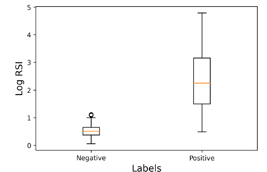
Figure 3 (from the paper). Boxplot of log RSI on the training set for the two groups.
Results.
- Median log RSI: about 0.5 in the no-residual group and about 2.25 in the residual group.
- The two “boxes” (interquartile ranges, IQR) do not overlap: the negative group lies in roughly 0.4–0.65, the positive group in roughly 1.5–3.15.
- Diagnosis on the test set: Accuracy 0.96 · Precision 0.86 · Recall 0.95 · F1 0.91.
Analysis.
- RSI is a strong discriminative feature. The distance between the two medians (~1.75 log units) is much larger than the IQR width of either group. Almost every negative case has log RSI below 1, while 75% of positive cases have log RSI above 1.5.
- The gray zone is around log RSI 0.5–1.1. The lower whisker of the positive group reaches down to ~0.5, overlapping the upper part of the negative group (upper whisker ~1 and a few outliers ~1.1). These are cases with very little residual thyroid tissue and weak uptake. They may explain why Precision (0.86) is lower than Recall (0.95): the decision threshold sits at the low end of the gray zone, so the model rarely misses cases but accepts some false positives.
- A Recall of 0.95 fits the clinical priority. Missing a case with residual tissue is more dangerous than sending a patient for further testing. For suspicious cases, physicians can still use TSH and Thyroglobulin (Tg) as well.
- The positive group's distribution is very wide (log RSI 0.5–4.8, meaning RSI values differ by tens of times). This makes biological sense, since the amount of residual thyroid tissue ranges from a few small fragments to an entire lobe. It is also why a log scale is appropriate: it compresses the large range of values and makes the distribution more balanced for the logistic model.
Experiment 2: Is DETR really better than CNNs without the preprocessing trick?
Question. Does DETR's advantage in spatial relationships show when all models receive only the original image (1 brightness level)?
Method. Train DETR, Faster R-CNN and YOLOv7 on the original images and measure per-class [email protected] on the test set (the “1 brightness level” rows of Table III).
Results.
| Model (1 brightness level) | Thyroid [email protected] | Shoulder [email protected] | [email protected] |
|---|---|---|---|
| DETR | 0.246 | 0.120 | 0.183 |
| Faster R-CNN | 0.375 | 0.079 | 0.227 |
| YOLOv7 | 0.00088 | 0 | 0.00044 |
Analysis.
- The shoulder is the hardest class for every model. On the original image the shoulders are nearly invisible, so shoulder mAP is low for all three models. Even so, DETR still detects the shoulders best (0.120 versus 0.079 for Faster R-CNN), consistent with the hypothesis: without local features, the model has to rely on position relative to the neck and head, and attention does this better.
- For the thyroid, Faster R-CNN is better. Residual thyroid is a small bright spot with clear local features. This is the strength of a CNN with FPN. The result matches the general understanding that the original DETR is not strong on small objects.
- YOLOv7 collapses completely (mAP ≈ 0) on the original images. Most likely, YOLO's anchors and label assignment cannot find meaningful positive samples when the image is almost black, so the model learns nothing. This is an example showing that input quality matters more than architecture.
- Takeaway from this experiment: at the original-image level, no model is usable in practice. DETR's advantage shows only on the shoulders, and the shoulder is precisely the denominator of RSI. That leads to the next experiment: how to make the shoulders “show up”.
Experiment 3: How many brightness levels are enough?
Question. Does stacking multiple brightness versions as channels help the model see the body outline and shoulders? How many levels are optimal?
Method. For each model, train with 1, 2, 3 and 4 brightness levels and measure [email protected] on the test set.
Results (Table III).
| Model | # Brightness levels | Thyroid [email protected] | Shoulder [email protected] | [email protected] |
|---|---|---|---|---|
| DETR | 1 | 0.246 | 0.120 | 0.183 |
| DETR | 2 | 0.330 | 0.150 | 0.240 |
| DETR | 3 | 0.447 | 0.161 | 0.304 |
| DETR | 4 | 0.660 | 0.200 | 0.430 |
| Faster R-CNN | 1 | 0.375 | 0.079 | 0.227 |
| Faster R-CNN | 2 | 0.555 | 0.238 | 0.396 |
| Faster R-CNN | 3 | 0.614 | 0.132 | 0.373 |
| Faster R-CNN | 4 | 0.660 | 0.128 | 0.394 |
| YOLOv7 | 1 | 0.00088 | 0 | 0.00044 |
| YOLOv7 | 2 | 0.523 | 0.014 | 0.268 |
| YOLOv7 | 3 | 0.674 | 0.092 | 0.383 |
| YOLOv7 | 4 | 0.513 | 0.131 | 0.322 |
xychart-beta
    title "[email protected] by number of brightness levels (Table III)"
    x-axis "Brightness levels" [1, 2, 3, 4]
    y-axis "[email protected]" 0 --> 0.5
    line "DETR" [0.183, 0.24, 0.304, 0.43]
    line "Faster R-CNN" [0.227, 0.396, 0.373, 0.394]
    line "YOLOv7" [0.00044, 0.268, 0.383, 0.322]
Line order: DETR, Faster R-CNN, YOLOv7.
Analysis.
- Brightening helps all three models, and helps most in the step from 1 to 2 levels: YOLOv7 goes from 0 to 0.268, Faster R-CNN from 0.227 to 0.396. This confirms that the initial bottleneck lies in the input data, not only in the architecture.
- Only DETR improves steadily and monotonically with the number of brightness levels (0.183 → 0.240 → 0.304 → 0.430). Each added channel is a different “view” of the same scene, and the attention mechanism can exploit combining information across channels and across distant regions.
- Faster R-CNN and YOLOv7 saturate early and then fluctuate. Faster R-CNN peaks at 2 levels, YOLOv7 at 3 levels. This “up then down” pattern suggests the CNN models start to overfit as the input gets more channels while the data has only 278 training cases. Note also that with a small test set, part of the fluctuation may just be statistical noise.
- At 4 brightness levels, DETR has the best overall mAP (0.430). The advantage comes from DETR balancing both classes: its thyroid score matches Faster R-CNN (0.66) while its shoulder score is clearly better (0.200 versus 0.128). Faster R-CNN with 2 levels has the highest Shoulder mAP in the table (0.238) but a weaker thyroid score (0.555).
- Cost trade-off. Each additional brightness level increases the number of input channels and the inference time. The paper chooses 4 brightness levels for the final configuration, since that is where DETR achieves its best result while the cost is still acceptable for 256×256 images.
Experiment 4: Select the model by mAP or by RSIA?
Question. During training, many checkpoints are saved. If we pick the checkpoint with the highest [email protected] on the validation set (the usual approach) and the checkpoint with the highest RSIA (the proposed metric), which gives the better final diagnosis?
Method. Use DETR with 4 brightness levels. Pick two checkpoints:
- Best normal model: the checkpoint with the highest [email protected] on validation;
- Best proposed model: the checkpoint with the highest RSIA (, ).
For each checkpoint, compute RSI from the predicted boxes on the test set, feed it into the same logistic model trained on RSI from ground truth boxes (Experiment 1), and measure F1. Also compare against direct ResNet-50 classification following the method of Phu et al. (NICS 2022).
Results (Table IV).
| Metric | Best proposed model (selected by RSIA) | Best normal model (selected by mAP) | Best ResNet-50 |
|---|---|---|---|
| RSIA | 0.457 | 0.436 | – |
| Thyroid [email protected] | 0.730 | 0.663 | – |
| Shoulder [email protected] | 0.604 | 0.570 | – |
| Shoulder [email protected] | 0.156 | 0.200 | – |
| Diagnostic F1 | 0.91 | 0.90 | 0.88 |
Analysis.
- Selecting by RSIA gives a better diagnosis, even though Shoulder [email protected] is lower. The model selected by RSIA has a Shoulder [email protected] of only 0.156 (versus 0.200), yet it is better on every other metric: RSIA, Thyroid [email protected], Shoulder [email protected] and, most importantly, F1.
- Why? For the shoulder, what matters for RSI is that the box sits in the right background region; it does not need to match the edges of the physician's subjective outline precisely. Because the shoulder region has fairly uniform intensity, shifting the box by a few pixels barely changes . Shoulder [email protected] heavily penalizes these “harmless” deviations, while Shoulder [email protected] and RSIA do not. This result also explains the choice of [email protected] for the shoulders in the metrics section.
- The general lesson: this is an example of the principle “select models using the metric closest to the final goal”. When the detector is only an intermediate step, optimizing directly for mAP can drift away from what we actually need (here, a correct RSI).
- Predicted boxes can almost replace the physician's boxes. F1 using DETR's boxes (0.91) equals F1 using the ground truth boxes in Experiment 1 (0.91). This means that in the diagnostic step, detector error barely degrades quality. That is a necessary condition for automating the whole workflow.
- Compared with ResNet-50 (F1 0.88): the “detection + RSI” approach beats direct classification and is also explainable (physicians see the boxes and the RSI value). Note that 0.88 is the ResNet-50 result within the SSP 2023 comparison, which differs from the ANT-POST figures in the NICS 2022 paper because the data and test sets are different.
Further analysis: reading the results critically
This section is commentary by the author of this post, to help readers understand the true scope of the results and to suggest directions for further work.
1. A small test set calls for confidence intervals
The test set has 39 cases. At this sample size, each case corresponds to about 2.6 percentage points of accuracy. The F1 difference between 0.91 and 0.90 in Experiment 4 is therefore equivalent to roughly one patient case.
To get a sense of the uncertainty, consider an illustrative example: 20 positive cases, of which the model catches 19 (Recall 0.95). The 95% Wilson confidence interval for Recall is then:
This interval is wide, so the 0.91 / 0.90 / 0.88 comparisons should be read as a consistent trend rather than statistically significant differences. Reasonable next steps are k-fold cross-validation, bootstrapping to obtain confidence intervals, and a McNemar test when comparing two models on the same test set.
2. Low absolute mAP is not necessarily bad
Shoulder [email protected] is only around 0.15–0.24, which sounds very low. But shoulder labels are inherently subjective (each physician outlines them differently), so the mAP ceiling that even another human annotator could reach may not be high. A worthwhile experiment would be to measure inter-observer agreement (inter-observer IoU) on the shoulder region, to know how far the model is from “human” level.
3. Factors that may affect RSI
- The inscribed ellipse is a simple geometric assumption. Residual thyroid tissue may be off-center, multifocal, or band-shaped. One could try replacing the ellipse with a segmentation mask or an intensity threshold within the box.
- Pixel sums depend on region area. If the shoulder box is larger than the thyroid box, grows with area. A variant worth trying is to use mean density so that RSI depends less on box size.
- Left and right shoulders: the data contain two shoulders. How they are combined (taking one shoulder, averaging both) will affect the stability of the denominator.
4. Directions for model improvements
- Newer DETR variants such as Deformable DETR, DINO and RT-DETR converge faster and handle small objects better than the original. They suit small datasets and small objects like the ones here.
- RSIA could be fed directly into training as a training signal (for example, by adding an RSI regression head), instead of being used only for checkpoint selection.
- Combine RSI with TSH and Tg in a multivariable model to handle the gray zone (log RSI 0.5–1.1).
- External validation on data from other hospitals and scanners is a mandatory step before clinical use.
Key concepts in brief
- Object detection: a task that both classifies and localizes: the model returns a list of (class, box, confidence).
- Bounding box: a rectangle around an object, described by its center and size or by two corners.
- Anchor boxes and NMS: Faster R-CNN and YOLO place a large number of template boxes (anchors) in advance and adjust them, then use NMS to remove duplicate boxes. DETR needs neither.
- Transformer and attention: an architecture originally designed for language processing. Each element “looks at” every other element and decides for itself where to focus.
- Object query: a learned vector in DETR; each query is responsible for “finding” at most one object.
- Hungarian algorithm: an algorithm that finds the one-to-one matching with the lowest total cost between two sets of elements.
- FPN (Feature Pyramid Network): combines features from multiple CNN layers to detect both large and small objects.
- Logistic regression: a linear classification model that turns a score into a probability using the sigmoid function.
- Checkpoint: a saved copy of the model's weights at a point during training.
Other foundational concepts (CNN, ResNet, transfer learning, overfitting, confusion matrix, AUC) are explained in the NICS 2022 post.
Related medical terms
- Total thyroidectomy: surgery to remove the entire thyroid gland, commonly performed for differentiated thyroid cancer.
- I-131 treatment (radioiodine ablation): after surgery, the patient swallows radioactive iodine I-131. Residual thyroid tissue and differentiated cancer cells take up the iodine and are destroyed by the radiation.
- I-131 SPECT scintigraphy: a gamma camera records where I-131 concentrates. Regions with remaining thyroid tissue appear bright on the image, helping assess whether treatment has removed all thyroid tissue.
- Uptake: how much radioactive material a tissue region retains, shown as photon counts on the image.
- TSH, Thyroglobulin (Tg): blood tests used alongside imaging for follow-up after treatment.
Frequently asked questions (FAQ)
What is RSI and why use the shoulder as the reference? RSI (Radioiodine Scan Index) is the ratio of total radioactive uptake in the thyroid region to that in the shoulder region on the same image. The shoulder is close to the neck but has no thyroid tissue, so it is a suitable background region. Dividing by the background removes the effect of the dose, scan timing and scanner.
Why not just use a CNN to classify directly? That approach (ResNet-50, NICS 2022 paper) gives F1 0.88 and is hard to explain. The “detection + RSI” approach gives F1 0.91, and physicians can see the regions the model outlines and the RSI value to check for themselves.
How is DETR different from YOLO or Faster R-CNN? DETR uses a Transformer so that every region of the image can “see” every other region, and it directly predicts a set of objects via Hungarian matching, with no anchors or NMS. In this paper, DETR detects the shoulders (a region with almost no local features) better than the two CNN models.
Why brighten the images? The shoulders do not take up iodine, so they are nearly invisible on the original image. Brighter versions reveal the body outline, helping the model locate the shoulders. For DETR, mAP rises from 0.183 (1 brightness level) to 0.430 (4 brightness levels).
How is RSIA different from mAP? mAP measures whether predicted boxes overlap the ground truth boxes. RSIA measures whether the RSI computed from predicted boxes is close enough to the true RSI (log-RSI error ≤ ε). Selecting the model by RSIA gives better diagnostic results than selecting by [email protected].
Does this model replace physicians? No. It is a support tool: it outlines regions, computes RSI and offers a suggestion. For cases in the gray zone, physicians still need to combine TSH, Tg and clinical experience.
How to cite
Paper citation (IEEE):
M. L. Phu, T. T. Nguyen, T. V. Pham, T. H. Nguyen, D. T. Pham, M. D. Chu, C. T. Nguyen, Q. L. Tran, D. T. Nguyen, N. H. Le, H. S. Mai, T. N. Nguyen, T. P. Nguyen, Q. K. Le, and N. T. Dang, “Utilizing DETR model on SPECT image to assess remaining thyroid tissues post-thyroidectomy,” in Proc. SSP 2023, 2023, pp. 537–541.
BibTeX:
@inproceedings{phu2023detr,
  title     = {Utilizing DETR model on SPECT image to assess remaining thyroid tissues post-thyroidectomy},
  author    = {Phu, Minh Lai and Nguyen, Thanh Trung and Pham, Thanh Vinh and Nguyen, Thai Ha and Pham, Duc Thuc and Chu, Minh Duc and Nguyen, Chi Thanh and Tran, Quoc Long and Nguyen, Duc Thuan and Le, Ngoc Ha and Mai, Hong Son and Nguyen, Thi Nhung and Nguyen, Thi Phuong and Le, Quoc Khanh and Dang, Nam Thang},
  booktitle = {SSP 2023},
  pages     = {537--541},
  year      = {2023},
  publisher = {IEEE}
}
References used by the paper
- M. Matsuu-Matsuyama et al., “Age-dependent effects on radiation-induced carcinogenesis in the rat thyroid,” Scientific Reports, vol. 11, no. 1, p. 19096, 2021.
- Y. Guo et al., “Classification and diagnosis of residual thyroid tissue in SPECT images based on fine-tuning deep convolutional neural network,” Frontiers in Oncology, vol. 11, 2021.
- M. L. Phu et al., “A deep learning method using SPECT images to diagnose remaining thyroid tissue post-thyroidectomy,” in 2022 9th NAFOSTED Conference on Information and Computer Science (NICS), IEEE, 2022, pp. 93–98.
- F. Abdolali et al., “Automated thyroid nodule detection from ultrasound imaging using deep convolutional neural networks,” Computers in Biology and Medicine, vol. 122, p. 103871, 2020.
- C.-Y. Wang, A. Bochkovskiy, H.-Y. M. Liao, “YOLOv7: Trainable bag-of-freebies sets new state-of-the-art for real-time object detectors,” arXiv:2207.02696, 2022.
- S. Ren et al., “Faster R-CNN: Towards real-time object detection with region proposal networks,” in Advances in Neural Information Processing Systems 28, 2015.
- N. Carion et al., “End-to-end object detection with transformers,” in Computer Vision – ECCV 2020, Springer, 2020, pp. 213–229.
- M. Everingham, S. A. Belongie, A. Zisserman, “Object detection performance evaluation,” 2007, pp. 1–8.
Additional references (not in the paper's reference list, added to explain concepts):
- A. Vaswani et al., “Attention is all you need,” in Advances in Neural Information Processing Systems 30, 2017. (positional encoding, attention)
- H. Rezatofighi et al., “Generalized intersection over union: A metric and a loss for bounding box regression,” in Proc. IEEE/CVF CVPR, 2019. (GIoU)
- T.-Y. Lin et al., “Feature pyramid networks for object detection,” in Proc. IEEE CVPR, 2017. (FPN)
- E. B. Wilson, “Probable inference, the law of succession, and statistical inference,” Journal of the American Statistical Association, vol. 22, no. 158, pp. 209–212, 1927. (Wilson confidence interval)
This article summarizes and explains the original paper for educational purposes. It is not medical advice. All numbers are taken from the IEEE SSP 2023 paper cited above; the “Further analysis” section is commentary by the author of this post.
Behind the notebook
Written by danielpham, AI Engineer.